| |
November 28, 2002
The current version of the F code can be found here.
I did some checks with the pulse fit. This is an example of a fitted pulse. Input are the
amplitude and T0 determined in the usual way. Since the
definition is different I shift T0 by 30 bins and scale
the amplitude by 5%. Additional parameters are: rise-time,
fall-time and pedestal. I run the 5 parameter fit only
with large pulses. From this run I determine the mean
for rise-time, fall-time and pedestal (calibration run).
This plot shows rise-time,
fall-time and pedestal determined for run 1037 (228 events)
and 1041 (300 events). In the 'normal' run only the amplitude
and T0 is free, T0 bound within +-200 bins of the start
value. I fit the 700 time bins shown in the plot, i.e.
200 bins before T0.
A comparison between
start and fit values.
The upper plots show the amplitude. The start value cannot
be larger than ~300. The fit can cope with overflows,
but the slope on the log-plot changes.
The middle plots are for large pulses, the offsets mentioned
above are chosen to get the maximum of these distributions
at 0 or 1. Sometimes the fit doesn't change the start
T0.
The lower plot are for small pulses (2<ampl<10).
Here the errors are rather large.
Scatterplot showing
correlations between fit and start parameters (top) and
between the differences of time and amplitude (bottom).
For large pulses differences in the amplitude are clearly
correlated with a shift in time. For smaller pulses this
is not so clear.
This plot shows the effect of PNoise on the diffusion
results for ArC02 data. Here is the plot
November 21, 2002
One plot to show that
the track fit in F works.
Fitted X0, phi; track width vs drift time; resolution row 5 and 6;
no cuts applied, i.e. no proper analysis, just proof of principal.
The routine does (should do) basically the same as the
JAVA code.
Differences:
phi(F) = -phi(JAVA)
The veto groups are in separate rows (11, 12) so they
don't interfere with the signal determination.
ScaleFactor to get the maximum amplitude from the integral
between timebins
50 - 150: F: 0.75; Java: 0.69
Net gain to get in the fit rElectrons from ADC counts:
F: 1.0; JAVA: 1.6E-4 * 2 * 3000 = 0.96
November 8, 2002
Scope pictures taken during data collection.
Taken at center of 19,
strips 15 to 18
Taken at center of 19,
strips 19 to 22
Taken at center of 20, single event
Taken at center of 20, 128 event
average
Taken at edge 19,20, single
event
Taken at edge 19,20, 128 event
average
The following plots are show the same distributions as the runs from Nov 7 except
the bin size has been changed. It is now 40 bins per mm instead of 50 bins per
mm.
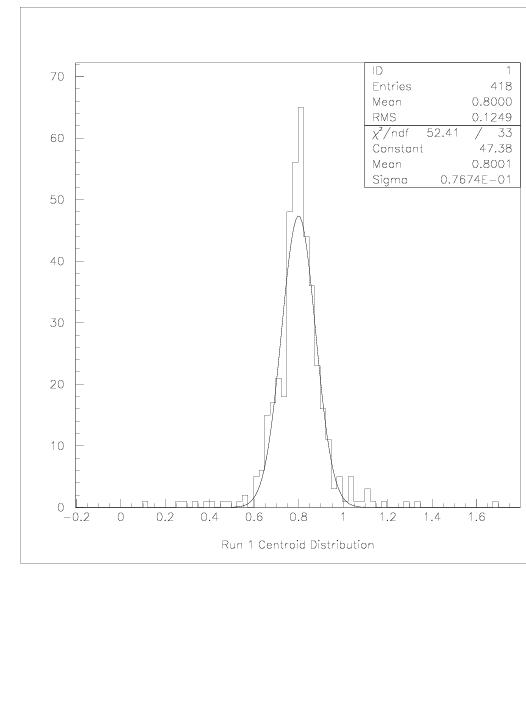
Run 1, edge 18/19
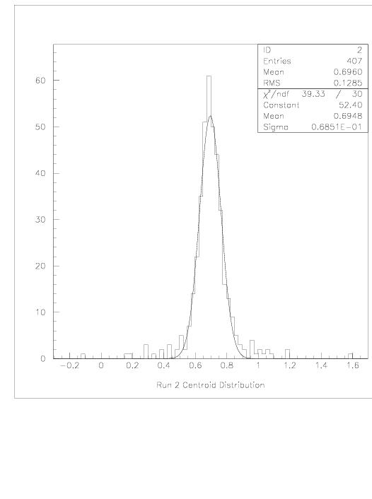
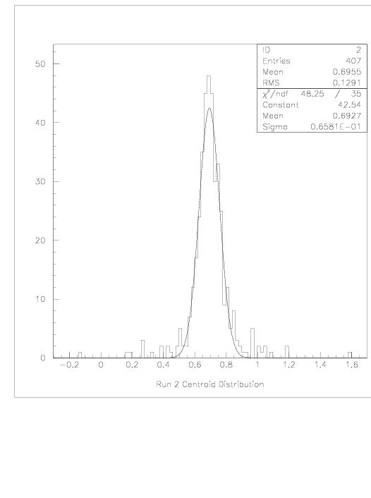
Run 2, 100 microns in
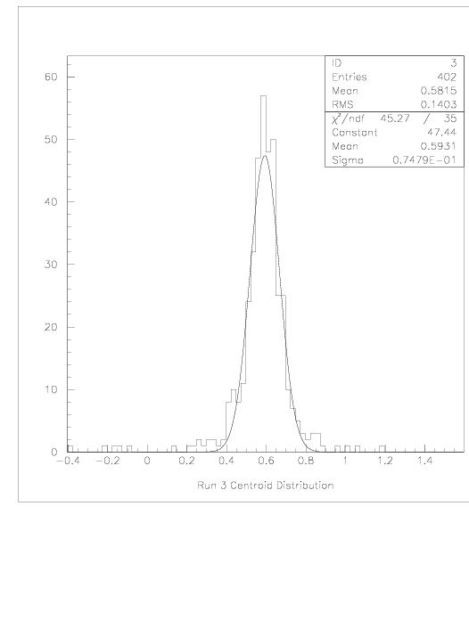
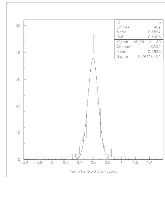
Run 3, 200 microns in
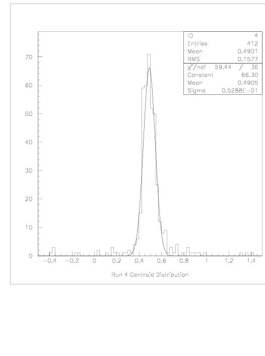
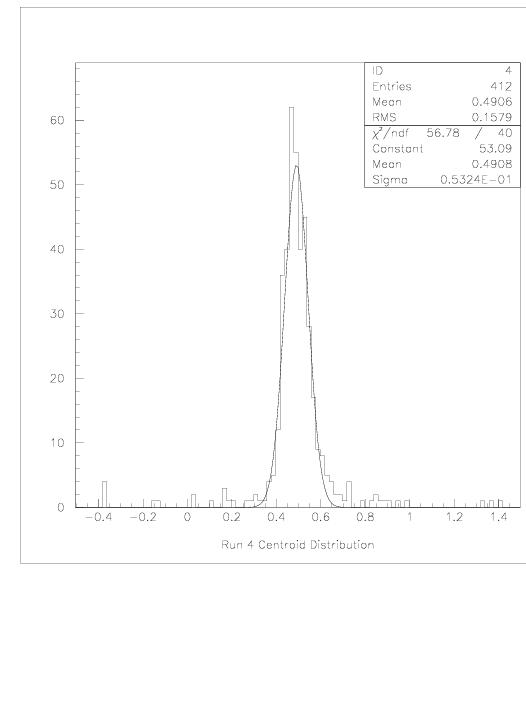
Run 4, 300 microns in
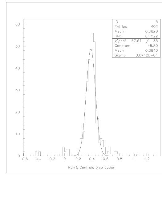
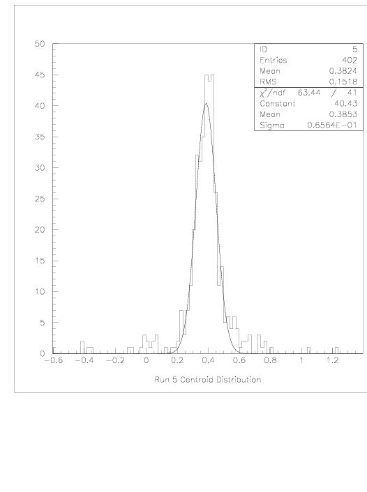
Run 5, 400 microns in
Run 6, 500 microns in
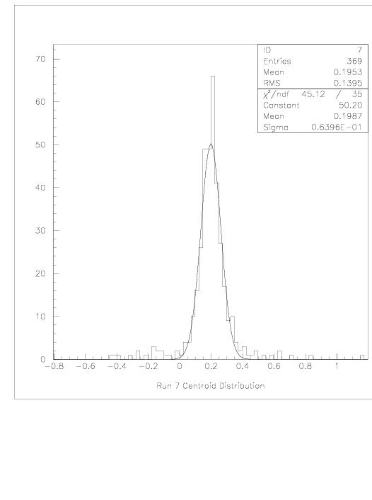
Run 7, 600 microns in
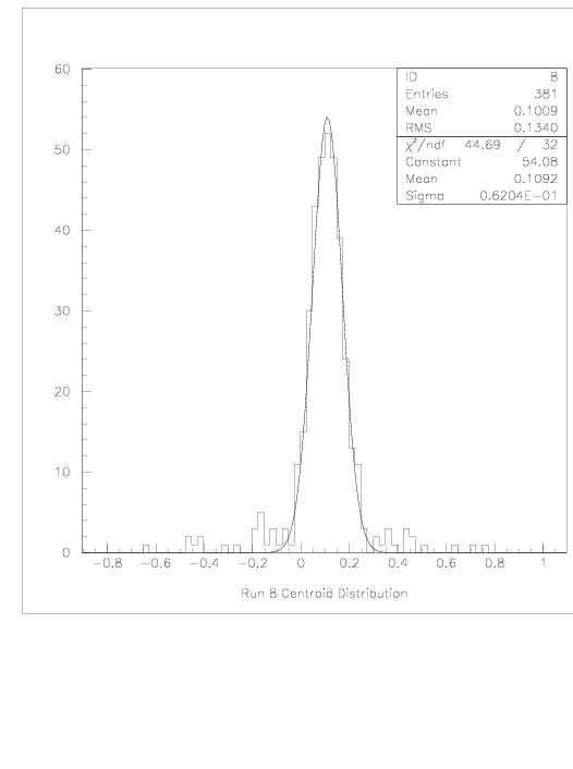
Run 8, 700 microns in
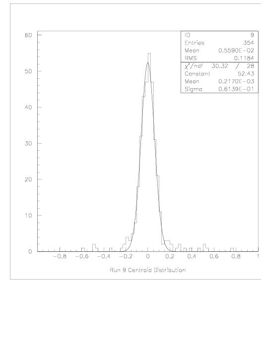
Run 9, center of 19
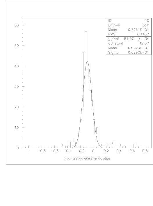
Run 10, 900 microns in
Run 11, 1000 microns in
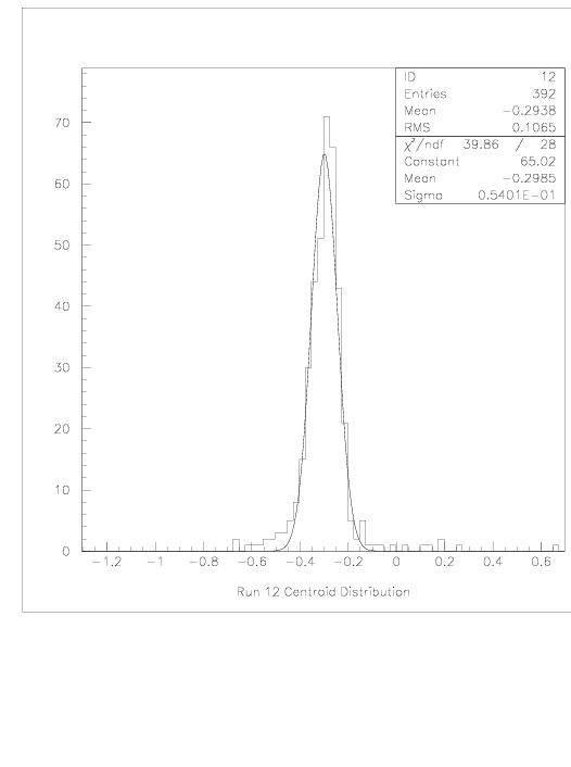
Run 12, 1100 microns in
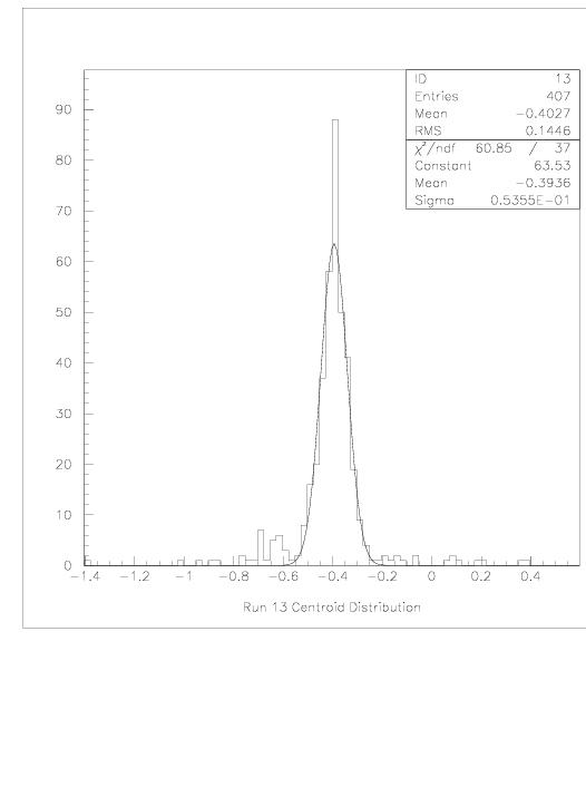
Run 13, 1200 microns in
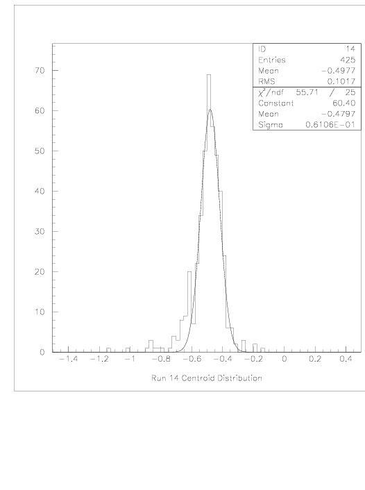
Run 14, 1300 microns in
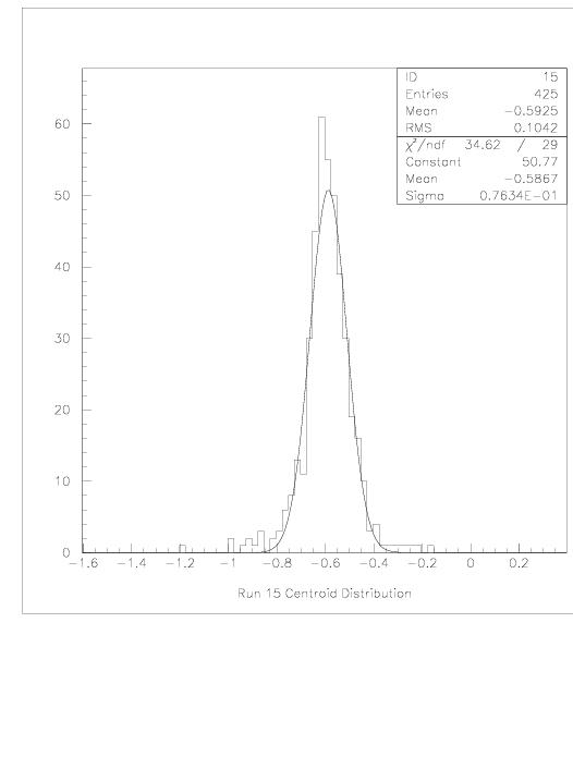
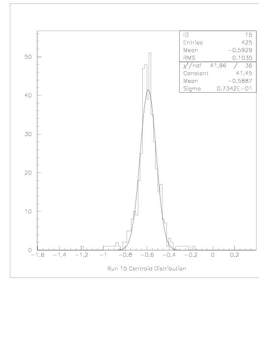
Run 15, 1400 microns in
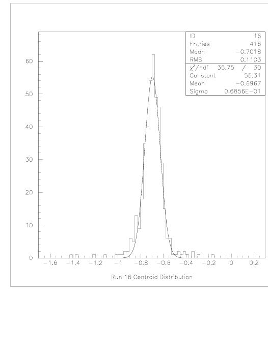
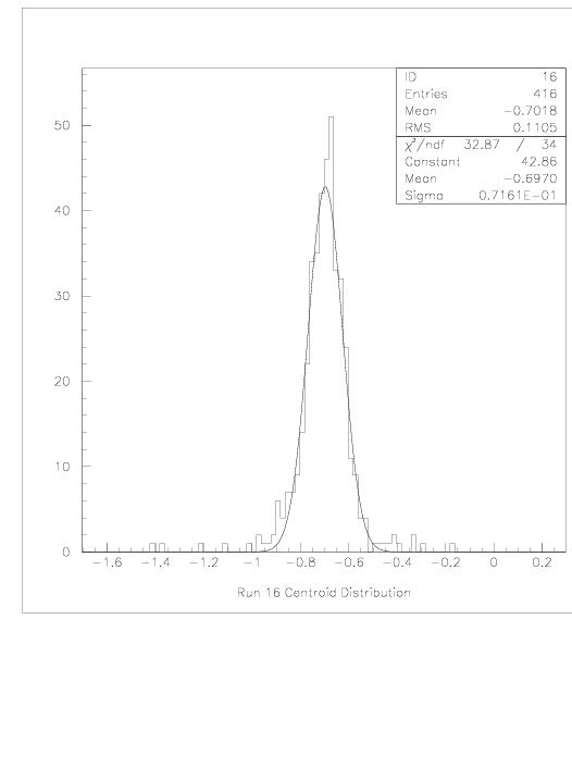
Run 16, 1500 microns in
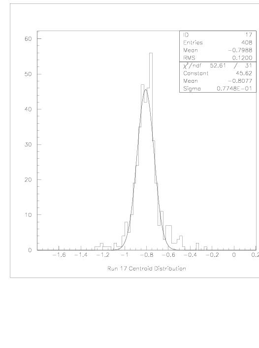
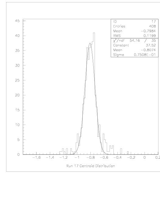
Run 17, edge 19/20
The following plot displays the residual and the resolution.
Residual/Resolution
November 7, 2002
The following plot shows averaged waveforms for a data run collected on the edge
of pads 18 and 19. The channels refer to their respective pad. The plots on
the left hand side show the average waveform with the fit through it. The right
hand side shows the fit reconstructed from the coefficients returned from the
program.
Average waveform with reconstructed fit.
With our new test cell data, we have been able to calculate calibration curves.
There are two curves in this pdf file.
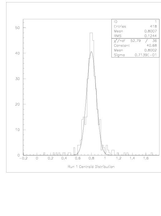
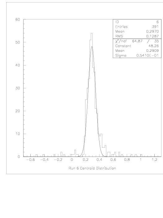
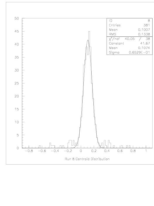
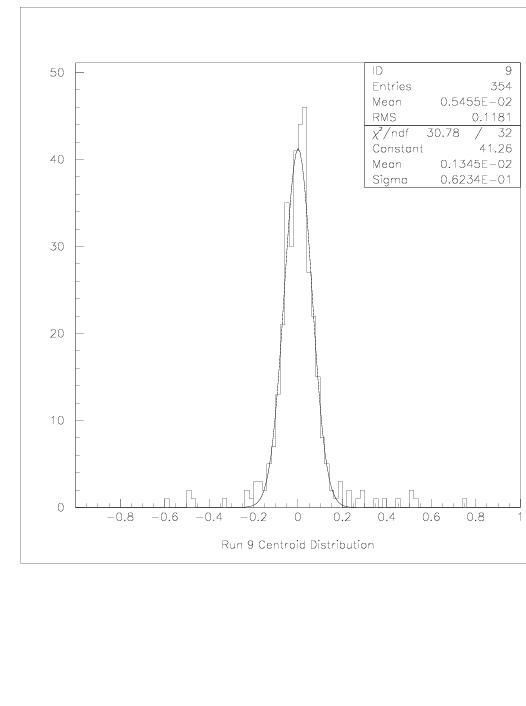
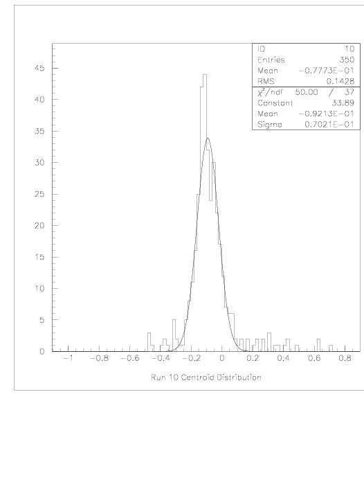
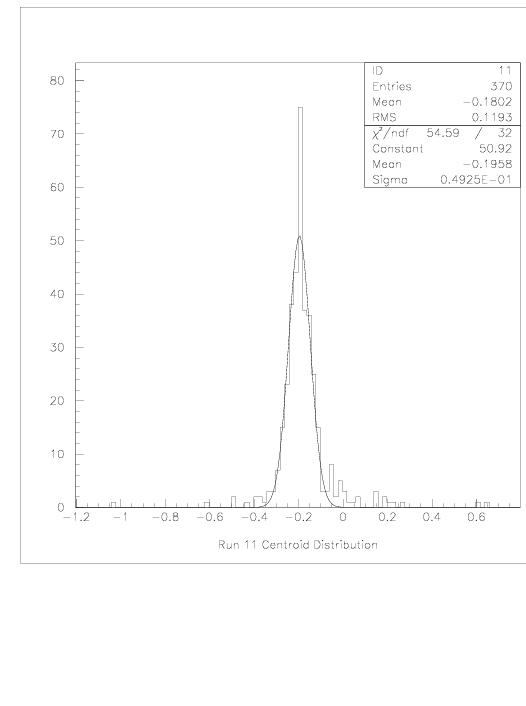
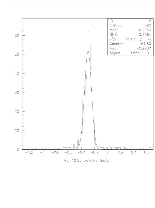
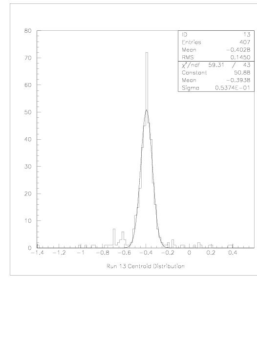
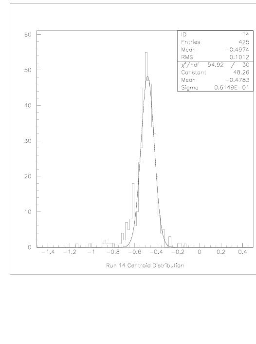
One strip was scanned from edge to edge with the test cell. After fitting the
amplitude, a centroid was determined. Using the calibration, the calculated centroid
position is converted to the event position. We have made the following distributions.
The x-axis in all of the plots is the normalized position in mm. All of the plots
except the plot of runs 1 to 4 come from a 500 event analysis. The other plot
came from 1000 event analysis. There isn't a 500 event plot due to the fits applied
in the 500 event analysis was nonsense because of calibration problems.
Run plots were updated on November 8, 2002 with a better calibration curve.
Run 1, edge 18/19
Run 2, 100 microns in
Run 3, 200 microns in
Run 4, 300 microns in
Run 5, 400 microns in
Run 6, 500 microns in
Run 7, 600 microns in
Run 8, 700 microns in
Run 9, center of 19
Run 10, 900 microns in
Run 11, 1000 microns in
Run 12, 1100 microns in
Run 13, 1200 microns in
Run 14, 1300 microns in
Run 15, 1400 microns in
Run 16, 1500 microns in
Run 17, edge 19/20
The following two plots show the difference between our calcuated position and
the true position.
Sigma vs Beam Position
Mean Position vs Beam Position
TPC analysis:
General overview for ArCO2 and P10 (X0, Phi, t0, Dt)
Dt is the time difference between the average of the
upper 4 rows and the lower 4 rows ~ theta
Resolution plots for ArCO2 and P10:
upper 4 plots for row 4, lower 4 plots for row 5
small Dt (ArCO2: < 500ns, P10: <
150ns)
page 1: small t0 (ArCO2: < 8000ns, P10: < 3300ns)
4 regions in |phi| (< 0.1 < 0.22 < 0.40 <)
page 2: small |phi| (< 0.1) 4 regions in t0 (ArCO2: < 5000 < 8000 < 12500 < ,
P10: < 3300 <
3800 < 4500 <)
Diffusion for ArCO2 and P10 with small Dt (ArCO2: < 500ns,
P10: < 150ns) and small |phi|
(< 0.1)
October 31, 2002
Still no track fit in F but some statistics for seed tracks in run 1041. Events with two
seed tracks mainly have phi>0.5 . I found one 2-track event like this, the typical case looks like this. Events with more seed tracks are just high
multiplicity.
The problem with channel 13 is some
ringing. Events selected for the averages were in fact noise. This should not
be a serious problem for the analysis.
October 24, 2002
Test-cell:
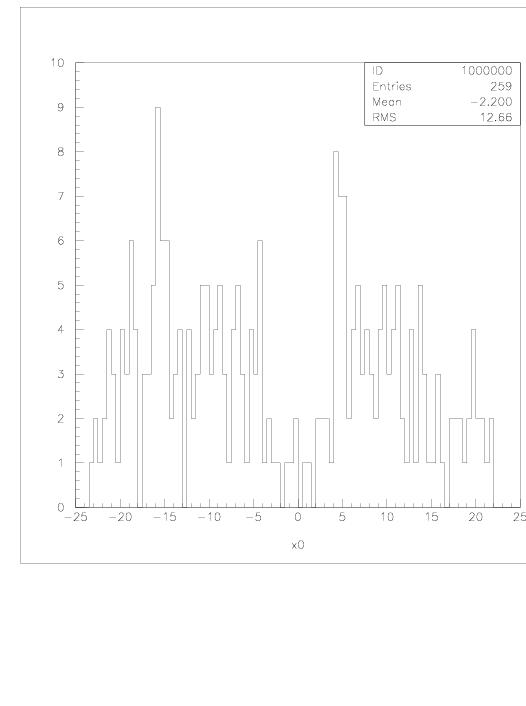
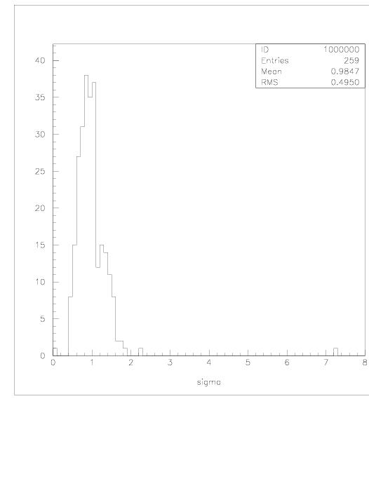
Distributions of the reconstructed x within strip 18 and at various edges. The centers look fine but the edges are
odd - the true value is between the two distributions.
including a noise level of 0.01 the fit improves. Here
are new distibutions for the width.
First plots with the Fortran routine, to prove the data
can be read and make sense and HBOOK is interfaced:
Profile distributions
for pedestals and pulse amplitudes of more than 10 (in
ADC counts).
Group 24 and 39 are filter; group 16 and 48 are veto.
Distributions for all groups of pedestals, amplitudes and
averaged pulse shapes (error
is spread).
October 17, 2002
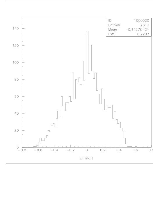
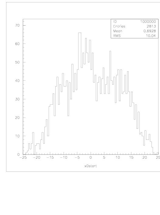
Distributions of x0, x0Start, phi, and phiStart
x0,x0Start for runs 1031-1035 (ArCO2)
Why does the fit fail mainly for small x0Start?
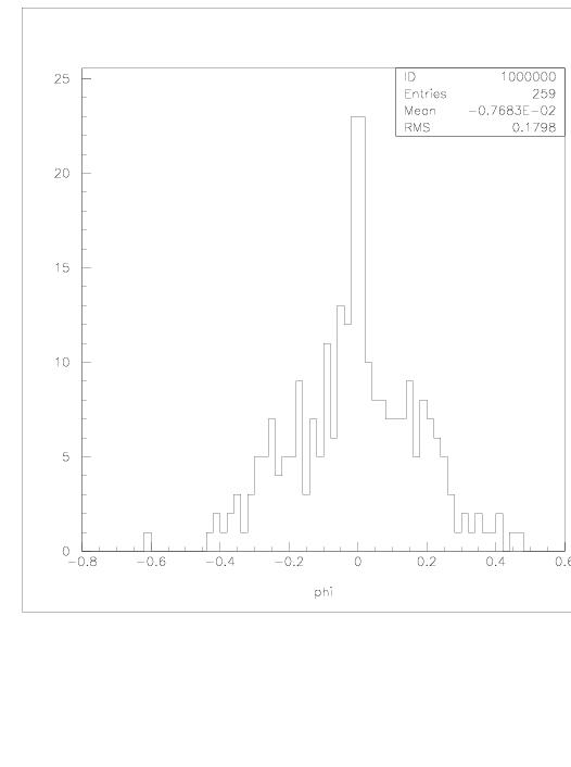
phi,phiStart for runs 1031-1035 (ArCO2)
Why does the fit fail less for large phi?
Why is phi asymmetric?
x0,x0Start for runs 1106-1110 (P10)
Why does the fit fail mainly for small x0Start?
phi,phiStart for runs 1106-1110 (P10)
Why does the fit fail less for large phi?
Why is phi asymmetric?
Distributions for failed fits for runs 1031-1035 (ArCO2)
phiStart for failed fits
x0Start for failed fits
Distributions for where the resolution fails but there is a fit for runs 1031-1035
(ArCO2)
phi for failed resolution x0
for failed resolution sigma for failed resolution
Distributions for sigma with straight tracks and varying drift distance
Sigma for changing drift distance
October 7, 2002
distributions for runs 1038-1043 (?)

phi, all events
what is the bump at phi < -0.5?
October 3, 2002
t0 distribution with shifted timing; the old t0=0 is a new
t0=1500.
Distribution starts at about 1400.
September 26, 2002
Distribution of number of electrons for
the pads used for tracking (i.e. not veto, not trigger)
x-axis: NELectron/1000. ; y-axis: # of pads
A first look at the resolution ntuple:
phi distribution
of all fitted tracks
resolution in row4 and row5
Top | Back
to Index |
|
